FMP
Instant Stock Intelligence: A Comprehensive Guide to FMPs Quote API
Nov 24, 2025
In today's world, quick and dependable information is vital across almost all sectors. This importance is particularly evident in trading, where the stakes are high and the margin between a profitable trade and a loss can be very narrow.
The FMP Stock Quote API offers a powerful solution for accessing detailed stock price information in a single request. It caters to both retail investors who have experience with APIs and investment firms aiming to keep track of their portfolio valuations. Additionally, users can set up notifications to alert them about market openings or major fluctuations in stock prices, enhancing their ability to respond to market changes effectively.
Endpoint Overview
To call the specific endpoint, you will need
- api-key: your api key (if you don't have one, you can obtain it by opening either a personal or an enterprise FMP account)
- symbol: the symbol you are interested in. In the example Python code below, we will request the stock quote of Apple stock (AAPL).
|
import requests symbol = 'AAPL' apikey = 'YOUR FMP API KEY' url = 'https://financialmodelingprep.com/stable/quote' params = {'apikey': apikey, 'symbol':symbol} r = requests.get(url, params=params) data = r.json() data |
By calling this url (https://financialmodelingprep.com/stable/quote), you will get a list of one dictionary with the following data:
|
[ { "symbol": "AAPL", "name": "Apple Inc.", "price": 268.47, "changePercentage": -0.48189, "change": -1.3, "volume": 45140079, "dayLow": 266.82, "dayHigh": 272.29, "yearHigh": 277.32, "yearLow": 169.21, "marketCap": 3967020108000, "priceAvg50": 252.2522, "priceAvg200": 224.3975, "exchange": "NASDAQ", "open": 269.795, "previousClose": 269.77, "timestamp": 1762549202 } ] |
As you will see, the response is a list that includes a dictionary with various datapoints. Let's see what each datapoint represents:
|
Field |
Description |
|
symbol |
Ticker symbol identifying the stock or security uniquely. |
|
name |
Full name of the company or financial instrument. |
|
price |
Current trading price of the stock in the market. |
|
changePercentage |
Percent change in stock price compared to previous close. |
|
change |
Absolute change in price since the last trading session. |
|
volume |
Total number of shares traded during the current session. |
|
dayLow |
Lowest price reached by the stock during today's trading day. |
|
dayHigh |
Highest price reached by the stock during today's trading day. |
|
yearHigh |
Highest price the stock has traded at in last year. |
|
yearLow |
Lowest price the stock has traded at in last year. |
|
marketCap |
Total market value of the company's outstanding shares. |
|
priceAvg50 |
Average stock price over the past 50 trading days. |
|
priceAvg200 |
Average stock price over the past 200 trading days. |
|
exchange |
Stock exchange where the security is listed and traded. |
|
open |
Opening price of the stock at the start of trading day. |
|
previousClose |
Final trading price at market close from previous day. |
|
timestamp |
Unix timestamp indicating the time of the quoted data. |
Let's explore what additional interesting data we can derive from these data points using their code snippet.
Momentum
One key insight from pricing data is identifying the stock's momentum: whether it's trending up or down. The following method shows a common approach: comparing a slow and a fast moving average. These averages are efficiently precomputed with this API, with the slow being 200 days and the fast being 50 days.
- If priceAvg50 > priceAvg200, it indicates an uptrend
- If priceAvg50 < priceAvg200, it signals a downtrend
- When price > priceAvg50 and priceAvg50 > priceAvg200, it confirms strong uptrend continuation.
- When price < priceAvg50 and priceAvg50 < priceAvg200, it confirms strong downtrend continuation
|
d = data[0] price = d.get('price') priceAvg50 = d.get('priceAvg50') priceAvg200 = d.get('priceAvg200')
if priceAvg50 > priceAvg200: trend_signal = "Uptrend (bullish momentum)" elif priceAvg50 < priceAvg200: trend_signal = "Downtrend (bearish momentum)" else: trend_signal = "Neutral/transition"
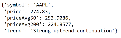
if price > priceAvg50 and priceAvg50 > priceAvg200: trend_signal = "Strong uptrend continuation" elif price < priceAvg50 and priceAvg50 < priceAvg200: trend_signal = "Strong downtrend continuation"
result = { "symbol": data[0].get("symbol") if data and isinstance(data, list) and data else None, "price": price if 'price' in locals() else None, "priceAvg50": priceAvg50 if 'priceAvg50' in locals() else None, "priceAvg200": priceAvg200 if 'priceAvg200' in locals() else None, "trend": trend_signal } print(result) |
Running the above code will produce an output based on the symbol and day. In the following example, you'll see that Apple stock is in a strong upward trend, as the price is above both moving averages, with the fast MA (50) above the slow MA (200):
Support and Resistance Levels
Another important aspect we can extract from this endpoint is the potential support or resistance levels. If the price is close to the yearHigh, the stock might be nearing resistance levels. If it's close to the yearLow, it could indicate support. The only variable we need to define is what "near" means. For this, we'll set a threshold of 3% as an example. See the code below:
|
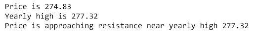
year_high = d.get('yearHigh') year_low = d.get('yearLow') threshold_percentage = 0.03 resistance_threshold = year_high * (1 - threshold_percentage) support_threshold = year_low * (1 + threshold_percentage) if resistance_threshold <= price <= year_high: sr_signal = f"Price is approaching resistance near yearly high {year_high:.2f}" elif year_low <= price <= support_threshold: sr_signal = f"Price is approaching support near yearly low {year_low:.2f}" else: sr_signal = "Price is not near significant resistance or support levels based on yearly range" print (f'Price is {price:.2f}') print (f'Yearly high is {year_high:.2f}') print(sr_signal) |
With Apple stock in a strong upward trend, the identified resistance level makes sense. As the price nears the yearly high, the script indicates there could be some resistance around that point.
Opening Gap
The opening gap percentage is calculated by the difference between yesterday's closing price and today's opening. This indicates that there might be some news that affected this gap overnight. Usually, those are surprises with earnings reports, news from rumours about mergers and acquisitions of the stock itself, to natural disasters and election results. Again, we should define what a significant gap will be for us. In our code example below, we set it as 3%.
|
open_price = d.get('open') previous_close = d.get('previousClose') threshold_percentage = 0.03
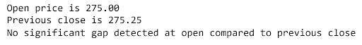
if open_price is None or previous_close is None or previous_close == 0: gap_signal = "Insufficient data to assess opening gap" else: price_diff = open_price - previous_close price_diff_pct = price_diff / previous_close if price_diff_pct >= threshold_percentage: gap_signal = f"Gap up detected: Open price {open_price:.2f} is higher than previous close {previous_close:.2f}" elif price_diff_pct <= -threshold_percentage: gap_signal = f"Gap down detected: Open price {open_price:.2f} is lower than previous close {previous_close:.2f}" else: gap_signal = "No significant gap detected at open compared to previous close"
print(f'Open price is {open_price:.2f}') print(f'Previous close is {previous_close:.2f}') print(gap_signal) |
In this case, the stock opened quite close to the previous day's close, so the script will inform us that there was no significant gap there.
Intraday volatility
By comparing the daily high and low, we can identify the intraday volatility, measuring price swing intensity and market activity. We can set a threshold so that if the day's high and low prices fall within this range, the script indicates that the day is not volatile. If they exceed the threshold, it will notify us about the volatility and the position of the current price. We will set this volatility threshold at 1%.
|
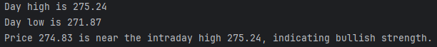
day_high = d.get('dayHigh') day_low = d.get('dayLow') print(f'Day high is {day_high:.2f}') print(f'Day low is {day_low:.2f}') closeness_threshold_pct = 0.01 if day_high is None or day_low is None or price is None: intraday_signal = "Insufficient data to assess intraday position" else: volatility_range = day_high - day_low # Check if the day's range is very tight relative to current price if price and price != 0 and volatility_range / price <= closeness_threshold_pct: intraday_signal = ( f"Very tight intraday range: High-Low = {volatility_range:.2f} " f"({(volatility_range / price) * 100:.2f}% of price)." ) elif volatility_range == 0: intraday_signal = "No intraday volatility detected as day high equals day low." else: position_in_range = (price - day_low) / volatility_range if position_in_range > 0.8: intraday_signal = f"Price {price:.2f} is near the intraday high {day_high:.2f}, indicating bullish strength." elif position_in_range < 0.2: intraday_signal = f"Price {price:.2f} is near the intraday low {day_low:.2f}, indicating bearish pressure." else: intraday_signal = f"Price {price:.2f} is within the intraday range {day_low:.2f} - {day_high:.2f}, neutral zone." print(intraday_signal) |
The output of the script above will show a message similar to this, indicating that the price is near the intraday high, suggesting the stock is on a bullish trend.
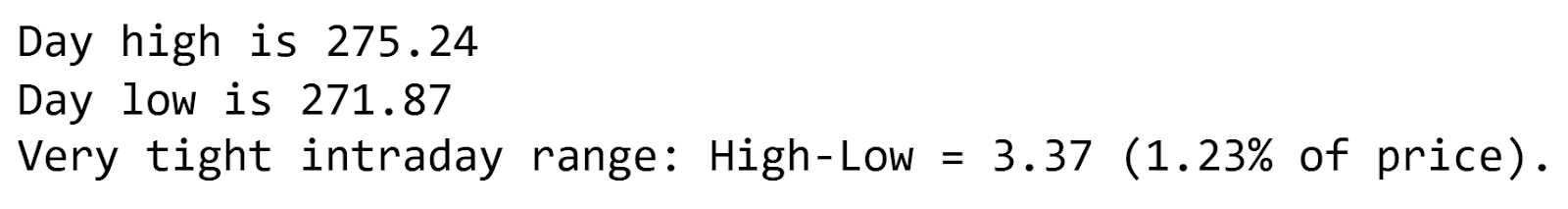
If we set the threshold to 1.5%, we see the following. The script indicates no significant volatility because the difference between low and high is only 1.23%. This highlights how important it is to establish a threshold that aligns with your trading style.
Advanced usage and plotting
Let's now visualise all these metrics together in a single plot. We will compare four stocks- Apple, Microsoft, Meta, and Google- and display their metrics side by side in four separate plots.
|
import pandas as pd import numpy as np import requests import matplotlib.pyplot as plt symbols = ['AAPL', 'MSFT', 'META', 'GOOG'] def fetch_quote(symbol): url = 'https://financialmodelingprep.com/stable/quote' params = {'apikey': apikey, 'symbol': symbol} r = requests.get(url, params=params) r.raise_for_status() data = r.json() return data[0] if isinstance(data, list) and data else {} def compute_metrics(d): price = d.get('price') priceAvg50 = d.get('priceAvg50') priceAvg200 = d.get('priceAvg200') open_price = d.get('open') previous_close = d.get('previousClose') day_high = d.get('dayHigh') day_low = d.get('dayLow') year_high = d.get('yearHigh') year_low = d.get('yearLow') # Momentum using moving averages if priceAvg50 is not None and priceAvg200 is not None: momentum = priceAvg50 - priceAvg200 else: momentum = np.nan # Gap percentage from open vs previous close if open_price is not None and previous_close not in (None, 0): gap = (open_price - previous_close) / previous_close else: gap = np.nan # Intraday volatility: normalized range if day_high is not None and day_low is not None and price not in (None, 0): volatility = (day_high - day_low) / price else: volatility = np.nan # Proximity to resistance (year high): smaller distance -> closer if year_high is not None and price is not None: resistance = (year_high - price) / year_high else: resistance = np.nan return { 'price': price, 'momentum': momentum, 'gap': gap, 'volatility': volatility, 'resistance': resistance } # Fetch and compute for all symbols records = [] for sym in symbols: d = fetch_quote(sym) m = compute_metrics(d) m['symbol'] = sym records.append(m) df_metrics = pd.DataFrame(records).set_index('symbol') # Plot 4 subplots: momentum, gap, volatility, resistance fig, axes = plt.subplots(2, 2, figsize=(12, 8), constrained_layout=True) ax1, ax2, ax3, ax4 = axes.ravel() # Momentum df_metrics['momentum'].plot(kind='bar', ax=ax1, color='steelblue', title='Momentum (50MA - 200MA)') ax1.axhline(0, color='gray', linewidth=0.8) # Gap (df_metrics['gap'] * 100).plot(kind='bar', ax=ax2, color='orange', title='Gap % (Open vs Prev Close)') ax2.axhline(0, color='gray', linewidth=0.8) ax2.set_ylabel('%') # Volatility (df_metrics['volatility'] * 100).plot(kind='bar', ax=ax3, color='seagreen', title='Intraday Volatility % (High-Low / Price)') ax3.set_ylabel('%') # Resistance proximity (df_metrics['resistance'] * 100).plot(kind='bar', ax=ax4, color='crimson', title='Proximity to Resistance % (Year High - Price) / Year High') ax4.set_ylabel('%') plt.show() |
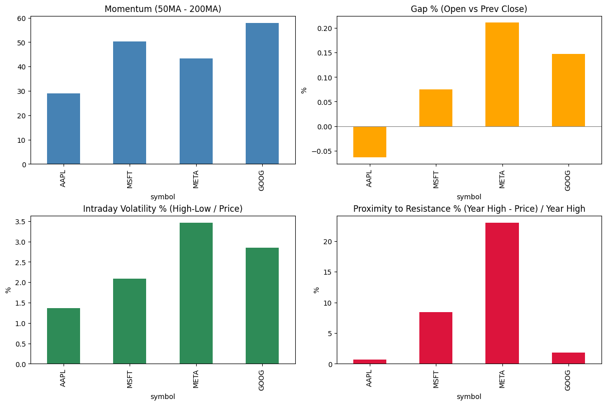
You can see in the example above, on just one screen, that
- Meta opened with the biggest upward gap, while Apple (as we observed earlier) opened with a small downward gap.
- In terms of momentum, Google is leading this metric.
- In terms of volatility, Meta is the most volatile during the trading day, which makes sense since it also had the highest gap. You can also observe some correlation between volatility and the gap - the larger the gap, the higher the intraday volatility.
- Regarding the year high approach, Apple is nearer to that zone (the smaller bar), indicating it might also face some resistance initially.
Other tips and tricks
Since FMP offers a wide range of endpoints, it's helpful to understand how its APIs function. This is an ideal chance to explore integrating this API with what we discussed earlier.
One approach is to start by dynamically fetching the entire universe of stocks through the FMP screener endpoint. This tool enables us to access all stock quotes for the:
- Technology Sector
- More than 100 billion in Market Cap
- At the NASDAQ exchange
And we will rank them based on how close they are to the year's high and low.
|
screener_url = f'https://financialmodelingprep.com/stable/company-screener' querystring = {"apikey":apikey, "marketCapMoreThan":100_000_000_000, "sector":"Technology", "country":"US", "exchange":"NASDAQ"} resp = requests.get(screener_url, querystring).json() df = pd.DataFrame(resp) tickers = df['symbol'].to_list() url = 'https://financialmodelingprep.com/stable/quote' results = [] # Ensure list_of_tickers exists; fallback to symbols if necessary # tickers = list_of_tickers if 'list_of_tickers' in locals() and list_of_tickers else [] for symbol in tickers: try: r = requests.get(url, params={"apikey": apikey, "symbol": symbol}) if r.status_code != 200: continue data = r.json() if not isinstance(data, list) or not data: continue q = data[0] price = q.get('price') yh = q.get('yearHigh') yl = q.get('yearLow') if price is None or yh in (None, 0) or yl in (None, 0): continue # Proximity percentages (smaller is closer) prox_high = (yh - price) / yh # 0 means at year high prox_low = (price - yl) / yl # 0 means at year low results.append({ "symbol": symbol, "price": price, "yearHigh": yh, "yearLow": yl, "prox_high": prox_high, "prox_low": prox_low }) except Exception: continue if not results: print("No valid quotes retrieved.") else: dfq = pd.DataFrame(results) # Closest to year high: smallest prox_high top_high = dfq.sort_values('prox_high').head(3).copy() # Closest to year low: smallest prox_low top_low = dfq.sort_values('prox_low').head(3).copy() print("Top 3 closest to Year High:") for _, row in top_high.iterrows(): pct = max(row['prox_high'], 0) * 100 print(f"{row['symbol']}: {pct:.2f}% below year high") print("\nTop 3 closest to Year Low:") for _, row in top_low.iterrows(): pct = max(row['prox_low'], 0) * 100 print(f"{row['symbol']}: {pct:.2f}% above year low") |
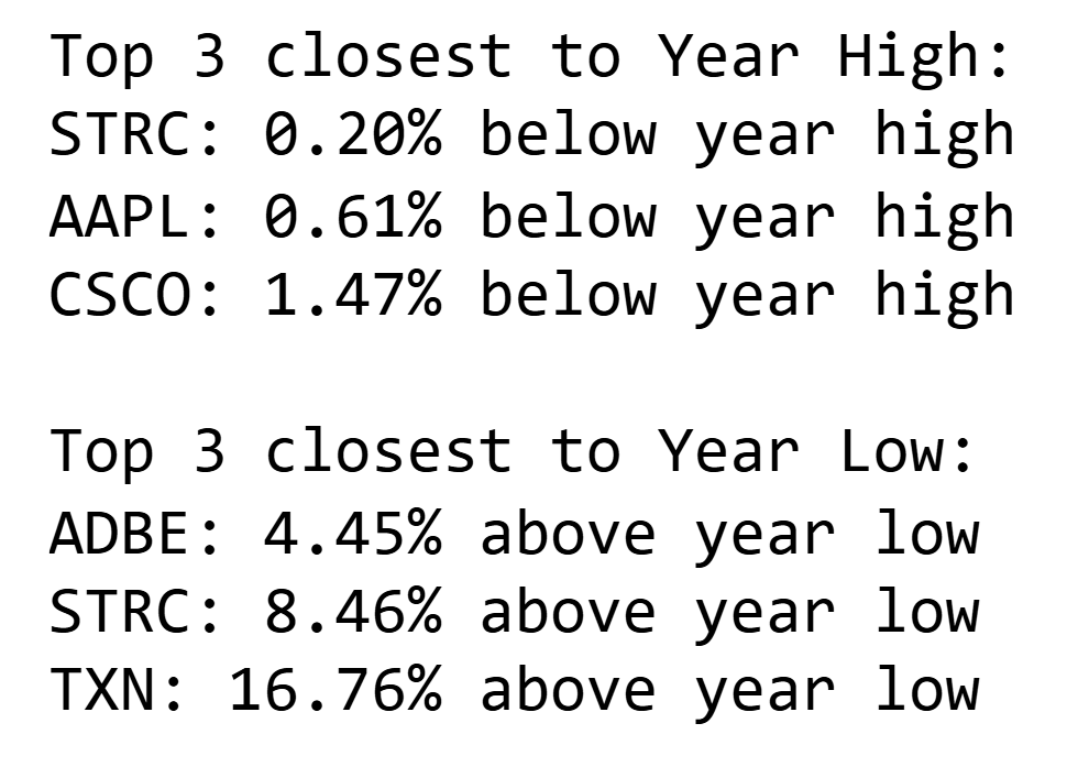
This output shows that the script highlights the three stocks nearest to the year's highest price and the three closest to the lowest. Currently, the Technology sector was mostly trending upward, which helps explain this trend.
- The first three stocks are quite close to their yearly highs, at 0.2% (Strategy Inc.), 0.61% (Apple Inc.), and 1.47% (Cisco Systems Inc.), indicating that there is a good probability the whole sector is at its yearly high.
- Regarding the stocks that are nearer to the year's low, we can see that Adobe and Texas Instruments are the closest (but still quite far from it).
- What is interesting is that Strategy Inc. falls into both categories. Investigating this stock, it appears to be a high dividend stock offering stable income, which clearly indicates that it does not fluctuate much.
Final Thoughts
The Stock Quote API is vital for financial data pipelines, offering fast access to detailed and reliable stock market data. Its comprehensive dataset allows developers and analysts to quickly retrieve key metrics like current prices, trading volume, and significant averages in a single request, supporting timely and informed decision-making.
This endpoint integrates seamlessly with other FMP APIs, such as screeners and company profiles, enabling users to easily retrieve, filter, and analyze stock universes. Together, they provide a powerful toolkit for building advanced market analysis and trading systems that respond to real-time data.
Explore the Stock Quote API today to elevate your applications with precise market insights. Integrating it will enhance your platform's capability to track stock movements and react quickly to market opportunities.

Top 5 Defense Stocks to Watch during a Geopolitical Tension
In times of rising geopolitical tension or outright conflict, defense stocks often outperform the broader market as gove...

Circle-Coinbase Partnership in Focus as USDC Drives Revenue Surge
As Circle Internet (NYSE:CRCL) gains attention following its recent public listing, investors are increasingly scrutiniz...

LVMH Moët Hennessy Louis Vuitton (OTC:LVMUY) Financial Performance Analysis
LVMH Moët Hennessy Louis Vuitton (OTC:LVMUY) is a global leader in luxury goods, offering high-quality products across f...